
As climate change melts sea ice, the US Geological Survey projects that two-thirds of the polar bear population will disappear by 2050, caused by malnutrition or starvation due to habitat loss. Photo: Andreas Weith/Wikimedia
Anirban DasGupta takes a look at NASA’s temperature data from the last 100 years:
The best scientists and the best human minds have been deliberately looking at extensive global and local temperature and climate data for the past several hundred years in search of an answer to one of mankind’s most acute and climacteric questions: is Earth’s climate and temperature profile slowly changing in a hostile and ominous direction for the continuity of our planet’s well-being? The National Academies of the US have written several detailed reports and draft reports on it (2013, 2015, 2016, 2017). Most of us are aware of the debates; but have we all personally looked at real data and tried to understand what it says? My intention here today is to satiate a personal curiosity: if we take US government’s global earth temperature data for the last fifty or hundred years, and pass them through a large battery of established statistical tests for stability, what do these tests show? Are the results mutually contradictory? Are they in fact more or less unanimous in their conclusions? Should I be seriously suspicious of the conclusions they reach? If so, why? I am writing this column as an observer and a reporter, and trying to not filter data through my personal lens or to interpret on behalf the reader.
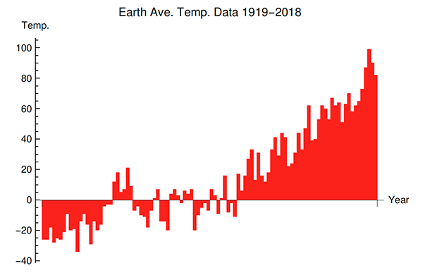
The data used here is NASA’s global average land-ocean temperature data for the 100-year period 1919–2018, available at giss.nasa.gov. The temperature data are reported with the 30-year period 1951–80 as the base, i.e., as deviations by year from the base period average, in the unit of 0.01ºC. Thus, a data value written as 12 means that the average land-ocean temperature of earth in that year was 0.12ºC above the average of the base period. The base period was chosen by NASA. In the sequel, I write t to denote the years, and xt the average temperature in year t. Here are the most basic summary statistics: mean of the series is 15.17, the median is 7, the variance is 1019.92, and the correlation between t and xt is 0.8966. It is quite interesting that temperature is so positively correlated with time as time moves forward. The 100 values of xt are listed chronologically in the box [below] for transparency as well as ease of verification and further analysis, if the reader desires.
Deviations from the base period 1951–80, in units of 0.01ºC:
−26, −26, −18, −28, −25, −26, −21, −9, −20, −19, −34, −14, −9, −16, −29, −14, −20, −16, −4, −3, −3, 12, 18, 5, 7, 21, 9, −7, −4, −10, −11, −18, −7, 1, 7, −14, −14, −20, 4, 7, 3, −2, 6, 4, 7, −20, −10, −5, −2, −7, 7, 3, −9, 1, 16, −8, −2, −11, 17, 6, 16, 27, 33, 13, 31, 16, 12, 18, 33, 41, 29, 44, 41, 22, 24, 31, 44, 33, 47, 62, 39, 40, 53, 62, 60, 53, 67, 62, 64, 51, 63. 70, 58, 62, 65, 73, 87, 99, 90, 82.
The hypothesis tested by a battery of tests is that earth’s average land-ocean temperature has been stable during the last 100 years. A rigorous statement is that the null hypothesis is that the sequence is iid from some distribution on the real line that has a density. Thus, no specific form of the density is assumed; we do not need to.
First, a time plot of the data; the x-axis represents the years chronologically, and the y-axis the corresponding temperatures (in hundredths of a degree).
And a histogram of the temperatures:
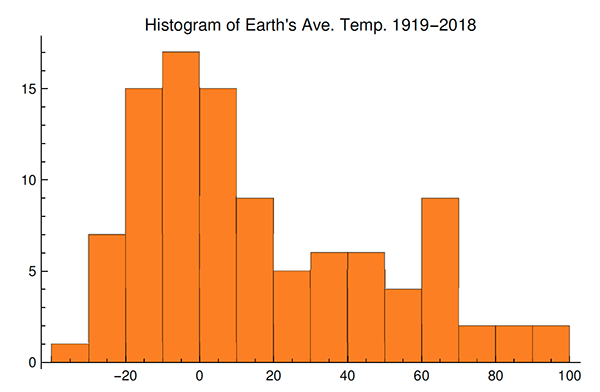
The histogram looks more like a bimodal mixture distribution than one homogeneous unimodal distribution.
And these are the tests that I conducted:
(a) Test based on U = Un, the number of upper records in the data; here n = 100 is the size of the dataset.
(b) Test based on L = Ln, the number of lower records in the data.
(c) Test based on R = Rn, the number of plus-runs or minus-runs in the data (a plus-run being an uninterrupted string of data values larger than the median of the data set).
(d) Bartel’s rank test based on the statistic M = ∑t=1n−1 (r(t+1) − rt )2,
where rt is the rank of the data value xt for year t among all the data. Thus, the minimum data value has rank one.
(e) Test based on the interarrival time lags Dr between successive upper records. For example, the 18th upper record was observed in 2015, and the 19th upper record was observed in 2016; and so, D19 = 1.
(f) A Kolmogorov–Smirnov test for equality of the temperature distribution in the first sixty years, 1919–78, and the last forty years, 1979–2018.
The tests in (a), (b), (c), (d), and (f) are based on the asymptotic distributions of the corresponding test statistics; these asymptotic distributions except in (f) are all normal and the asymptotic means and variances are known. Actually, even the exact means and variances are known for the record statistics Un, Ln and the run statistic Rn. The asymptotic distribution of the Kolmogorov–Smirnov two sample statistic is classic through the Donsker invariance principle and the theory of Brownian bridges. For case (e), the exact distribution of the record interarrival time Dr is known as an explicit combinatorial sum obtained through equating coefficients in generating functions. (All of these are quite classic, but I provide references at the end.)
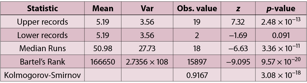
The table [below] shows the values of the test statistics and the associated two-sided p-values for each test based on the 100 data values.
For the record interarrivals test, the p-values for the interarrival times of the rth upper record for r = 2, 5, 8, 11, 14, 17, 19 are, respectively, 0.14, 0.03, 0.004, 0.0005, 6.1×10⁻⁵, 3.0 × 10⁻⁵, and 1.9 × 10⁻⁶. We note that the interarrival times demonstrate much lower p-values for the recent upper records and conventional p-values for the early upper records. Traditionally, the credibility of a null hypothesis has been questioned when the p-value is small, 0.001 already regarded as small by many. I ask the readers to interpret these findings as they wish.
I can think of a number of possible objections raised against this report, e.g.,
1. p-values are not meaningful and they should not be computed.
2. We already know that the sequence is not iid, but perhaps stationary.
3. The data should have covered a shorter time period.
4. One should look at many NASA data sets, not just the average land-sea temperature data set.
References
Let me close with some references: Arnold, Balakrishnan and Nagaraja, 1998; Bickel and Doksum, 2015; DasGupta, 2011; Del Barrio, Deheuvels and van de Geer, 2007; Gibbons and Chakraborti, 1992; Haigh, 2013; Katzenbeisser, 1990; Nevzorov, 2000; Port, 1993; Renyi, 1962; Resnick, 1973; Shorack and Wellner, 2009; Shorrock, 1973; Strawderman and Holmes, 1970.
Comments on “Anirban’s Angle: Earth’s temperature data”