Peter Diggle gave this Medallion Lecture at the ENAR meeting in March 2016.

Peter began his academic career in 1974 as Lecturer in Statistics at the University of Newcastle upon Tyne, UK. Between 1984 and 1988 he was Senior Research Scientist, then Principal Research Scientist, then Chief Research Scientist in the CSIRO Division of Mathematics and Statistics in Canberra. Since 1988 he has been at Lancaster University, where his current position is Distinguished University Professor of Statistics in the Faculty of Health and Medicine. He also holds Adjunct positions at Johns Hopkins, Yale and Columbia Universities, and is president of the Royal Statistical Society (2014–16). His research interests are in statistical methods for spatial and longitudinal data analysis and their applications in the biomedical and health sciences, with a particular focus on environmental and tropical disease epidemiology.

Model-Based Geostatistics for Prevalence Mapping in Low-Resource Settings

In low-resource settings, prevalence mapping plays an important role in determining priority areas for large-scale prevention and treatment programmes. Because disease registries are lacking, prevalence mapping relies on field data collected from prevalence surveys of communities within the region of interest. Only a small fraction of at-risk communities can be included in these surveys, and mapping at unsampled locations necessarily involves some form of interpolation or smoothing of the data. The precision of the interpolated maps can be improved by exploiting the availability of remotely sensed images that act as proxies for environmental risk factors.

A standard geostatistical model for data of this kind is a generalized linear mixed model,

$Y_i \sim$ Bin $\{m_i, P(x_i) \} $
log$[P(x_i)/ \{1−P(x_i)\} = z(x_i)′β + S(x_i) + U_i$,

where $Y_i$ is the number of positives in a sample of $m_i$ individuals at location $x_i$, $z(x)$ is a vector of spatially referenced explanatory variables, $S(x)$ is a spatially correlated Gaussian process and the $U_i$ are uncorrelated Gaussian random variables. The roles of $S(x)$ and $U_i$ are to account for spatially structured and unstructured variation, respectively, that is not explained by $z(x)$.

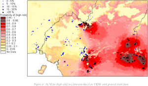
This model has been used in particular to assist the operation of pan-African control programmes for two vector-borne diseases, onchocerciasis (river blindness) and lymphatic filariasis (elephantiasis). The control strategy is based on prophylactic administration of a filaricide, Mectizan, to whole communities in affected areas. In this context, estimating prevalence at a particular location is less important than predicting whether prevalence exceeds a policy-relevant threshold. For example, the operation of the control programmes has been hampered by the recognition that people heavily infected with a third disease, Loa loa (eyeworm), are at risk of experiencing severe, occasionally fatal, adverse reactions to Mectizan. This has resulted in a policy that precautionary measures must be taken before the drug is administered in a community where prevalence of eyeworm is greater than 20%. Accordingly, the map (below) shows the predictive probability, at each location, that this threshold is crossed. The map effectively delineates areas that are “safe”, “unsafe” (predictive probabilities close to zero or one, respectively) and intermediate areas (in pink) where more information is needed.

Work is in progress on the following extension to the eyeworm problem. It is now known that those at risk of experiencing severe reaction to Mectizan are people whose blood is heavily infected with Loa loa parasites, more than 30,000 parasites per ml of blood. Determining infection levels routinely in the field is difficult. However the distribution of individual infection levels, $Y$, within a community is well described by a Weibull distribution,

$P(Y > y) = P$ exp $\{−(y/L)^\kappa \} : y ≥ 0,$

where $κ≈0.5$ and $(P, L)$ vary randomly between communities. Specifically, $S_1 (x) = log{P/(1−P)}$ and $S_2 (x) = log L$ can be modelled as a bivariate Gaussian process and the correlation between the two exploited to enable prediction of $P(Y>30,000)$ in a newly sampled community for which only prevalence data are available. Two general conclusions from this work are that in low resource settings: geostatistical modelling of prevalence data can deliver practical solutions to problems that would otherwise be intractable; and that predictive probability mapping is often a more useful inferential paradigm than either testing or estimation.

References

Diggle, P.J., Thomson, M.C., Christensen, O.F., Rowlingson, B., Obsomer, V., Gardon, J., Wanji, S., Takougang, I., Enyong, P., Kamgno, J., Remme, H., Boussinesq, M. and Molyneux, D.H. (2007). Spatial modelling and prediction of Loa loa risk: decision making under uncertainty. Annals of Tropical Medicine and Parasitology, 101, 499–509.

Zoure, H.G.M., Noma, M., Tekle, A.H., Amazigo, U.V., Diggle, P.J., Giorgi, E. and Remme, J.H.F. (2014). The geographic distribution of onchocerciasis in the 20 participating countries of the African Programme for Onchocerciasis Control: 2. Pre-control endemicity levels and estimated number infected. Parasites and Vectors, 7, 326

Schlueter, D.K., Ndeo-Mbah, M.L., Takougang, I., Ukety, T., Wanji, S., Galvani, A.P. and Diggle, P.J. (2016). Using community-level prevalence of Loa loa infection to predict the proportion of highly-infected individuals: statistical modelling to support lymphatic filariasis elimination programs. PLoS Neglected Tropical Diseases (submitted).