Contributing Editor Dimitris Politis writes:

Consider the standard setup where $X_1,\dots ,X_n$ are i.i.d. from distribution $F$ with mean $\mu =E{X}_i$, variance ${\sigma }^2=E(X_i-\mu {)}^2>0$, skewness $\gamma =E(X_i-\mu {)}^3/{\sigma }^3$, and kurtosis $\kappa =E(X_i-\mu {)}^4/{\sigma }^4$ assumed finite. As usual, define the sample mean $\overline{X}=\frac{1}{n}\sum _{i=1}^n{X}_i$, the sample variance ${\hat{\sigma }}^2=\frac{1}{n-1}\sum _{i=1}^n(X_i-\overline{X}{)}^2$, and the $t$-statistic $T=\sqrt{n}(\overline{X}-\mu )/\hat{\sigma }$.

At the beginning of the 20th century, the classical theory for the $t$ and ${\chi }^2$ tests was developed by the statistical pioneers W.S. Gosset (“Student”), R.A. Fisher, etc. These were undoubtedly major breakthroughs at the time but are intimately tied to the assumption that $F$ is Gaussian which is often hard to justify. Indeed, the true sampling distribution of $T$ and $(n-1){\hat{\sigma }}^2$ can be quite different from the textbook $t_{n-1}$ and $\sigma {\chi }_{n-1}^2$ distributions respectively even under moderate non-normality.

Skewness and the $t$-statistic

Nowdays that samples are typically large, practitioners may be reluctant to start out with such a restrictive assumption as normality, relying instead on a Central Limit Theorem (CLT). It is well known that the accuracy of the CLT for $\overline{X}$ depends on the skewness of the data. Under regularity conditions, an Edgeworth expansion yields [Eq. 1]
$P(\sqrt{n}(\overline{X}-\mu )/\sigma \le x)=\mathrm{\Phi }(x)+b(x)\gamma /\sqrt{n}\frac{c(x)\gamma }{\sqrt{n}}+O(1/n)$
for all $x$, where $\mathrm{\Phi }(\cdot )$ is the standard normal distribution, and $b(\cdot )$ a bounded function. Eq.[1] indicates that the distribution of $\overline{X}$ has a skewness of order $\gamma /\sqrt{n}$ that is not captured in the symmetric shape of the limit distribution.

What is perhaps lesser known is that skewness induces a strong dependence between the numerator and denominator of the $t$-statistic thereby shedding doubt on the accuracy of the $t$-tables; Hesterberg \cite{h} brings out this point.

Figure 1 depicts a scatterplot of $\overline{X}$ vs. $\hat{\sigma }$ based on 250 simulated samples each of size $n=30$ from $F=\frac{1}{2}{\chi }_2^2$, i.e., exponential; the correlation between $\overline{X}$ and $\hat{\sigma }$ is unmistakeable.

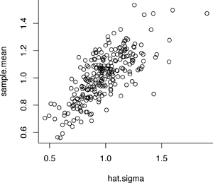
Figure 1: Scatterplot of $\overline{X}$ vs. $\hat{\sigma }$ based on 250 exponential samples each of size $n=30$

One might think that this is a phenomenon particular to the exponential distribution where $\overline{X}$ and $\hat{\sigma }$ estimate the same parameter. In fact, the phenomenon holds true for any skewed distribution $F$, and the correlation persists regardless of sample size. To elaborate, the $\delta$-method implies Corr$(\overline{X},\hat{\sigma })\approx$ Corr$(\overline{X},{\hat{\sigma }}^2)\to \gamma /\sqrt{\kappa -1}$ as $n\to \mathrm{\infty }$. When $F$ is exponential, $\gamma =2$, $\kappa =9$, and Corr$(\overline{X},\hat{\sigma })\approx 0.7$. Incidentally, this large-sample correlation calculation shows as a by-product the nontrivial general inequality ${\gamma }^2\le \kappa -1$ which is sharper than what Littlewood’s inequality implies; see p.~643 of DasGupta \cite{Das} with $r=4,s=3$ and $t=2$. Interestingly, when $F$ is Bernoulli($p$), the identity ${\gamma }^2=\kappa -1$ holds for any $p\in (0,1)$.

An Edgeworth expansion for the $t$-statistic yields [Eq.2]
$P(\sqrt{n}(\overline{X}-\mu )/\hat{\sigma }\le x)=\mathrm{\Phi }(x)+c(x)\gamma /\sqrt{n}\frac{c(x)\gamma }{\sqrt{n}}+O(1/n)$
where $c(\cdot )$ is another bounded function. Figure 2 shows the true density of $T$ obtained via Monte Carlo simulation from an exponential sample of size $n=30$ with the $t_{29}$ density superimposed. The true density is skewed left although visually this might not appear particularly striking. However, the true 2.5\% and 5\% quantiles of $T$ are $-2.84$ and $-2.28$ respectively that are poorly approximated by the corresponding $t_{29}$ quantiles $-2.04$ and $-1.70$.

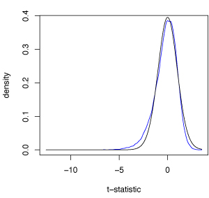
Figure 2: True density of the $t$-statistic calculated from an exponential sample of size $n=30$ (in blue) with the $t_{29}$ density superimposed (in black).

Luckily, Efron’s bootstrap can be applied to the studentized sample mean, i.e., the statistic $T$, yielding a better approximation. As expounded upon by Hall, the studentized bootstrap captures the skewness, i.e., [Eq.3]
$P^{\ast }(\sqrt{n}({\overline{X}}^{\ast }-\overline{X})/{\hat{\sigma }}^{\ast }\le x)=\mathrm{\Phi }(x)+c(x)\gamma /\sqrt{n}\frac{c(x)\gamma }{\sqrt{n}}+O_P(1/n)$
where ${\overline{X}}^{\ast }=\frac{1}{n}\sum _{i=1}^n{X}_i^{\ast }$, ${\hat{\sigma }}^{\ast }=\sqrt{\frac{1}{n-1}\sum _{i=1}^n(X_i^{\ast }-{\overline{X}}^{\ast }{)}^2}$, and the re-sample $X_1^{\ast },\dots ,X_n^{\ast }$ is obtained by i.i.d. sampling from the empirical distribution of $X_1,\dots ,X_n$. Let $q^{\ast }(\alpha )$ denote the $\alpha$-quantile of the LHS of Eq.[3] which serves as an estimator of $q(\alpha )$, the $\alpha$-quantile of the LHS of Eq.[2]. In the exponential example with $n=30$, the expected values of $q^{\ast }(0.025)$ and $q^{\ast }(0.050)$ are (approximately) $-2.90$ and $-2.31$, i.e., very close to the true ones.

Kurtosis and asymptotic failure of the ${\chi }^2$ test

The saving point for Student’s $t$ approximation is that $\hat{\sigma }\to \sigma$ almost surely as $n\to \mathrm{\infty }$. Since a constant is independent to all random variables, $\hat{\sigma }$ will gradually, i.e., asymptotically, become independent to $\sqrt{n}(\overline{X}-\mu )$, and the $t$ distribution will become standard normal. Hence, Student’s $t$ approximation to the distribution of $T$ is asymptotically valid for non-Gaussian data (with finite variance).

The ${\chi }^2$ test does not even have this excuse: it is asymptotically {\it invalid} when $\kappa \ne 3$. This might appear surprising since the ${\chi }_m^2$ distribution is asymptotically normal when $m$ is large; however, it has the wrong asymptotic variance. To see why, let $Y_i=(X_i-\mu {)}^2$ and $\overline{Y}=\frac{1}{n}\sum _{i=1}^n{Y}_i$. Then, a CLT on the i.i.d.~variables $Y_1,\dots ,Y_n$ yields [Eq.4]
$P(\sqrt{n}(\overline{Y}–{\sigma }^2)\le x)\to \mathrm{\Phi }(x/\tau )\text{as}n\to \mathrm{\infty }$
where ${\tau }^2=(\kappa -1){\sigma }^4$. But $\sum _{i=1}^n(X_i-\overline{X}{)}^2=\sum _{i=1}^n(X_i-\mu {)}^2+V_n$ with $V_n=O_p(1)$, i.e., bounded in probability. Hence, Eq.[4] implies Eq.[5]
$P(\sqrt{n}({\hat{\sigma }}^2–{\sigma }^2)\le x)\to \mathrm{\Phi }(x/\tau )\text{as}n\to \mathrm{\infty }$.

Recall that a ${\chi }_m^2$ variable has mean $m$ and variance $2m$. Hence, the ${\chi }_{n-1}^2$ approximation to the distribution of $(n-1){\hat{\sigma }}^2/{\sigma }^2$ is associated with a large sample approximation analogous to Eq.[5] with ${\tau }^2$ replaced by $2{\sigma }^4$; but this is only admissible when the kurtosis $\kappa$ equals 3 as it does in the Gaussian case. If $\kappa >3$, the ${\chi }^2$ approximation underestimates the variance of ${\hat{\sigma }}^2$ leading to confidence intervals with smaller level than nominal. In the exponential case, the ${\chi }^2$ approximation effectively estimates the variance of ${\hat{\sigma }}^2$ to only be $1/4$ of what it truly is.

Eq.[5] is valid in general but in order to be practically useful for tests and confidence intervals it needs a consistent estimate of ${\tau }^2$ to be plugged in, e.g., letting ${\hat{\tau }}^2=(\hat{\kappa }-1){\hat{\sigma }}^4$ where $\hat{\kappa }$ is the sample kurtosis. Furthermore, finite-sample accuracy can be improved via a skewness-reducing transformation such as the logarithmic; Eq.[5] together with the $\delta$-method yields Eq.[6]
$P(\sqrt{n}(\log {\hat{\sigma }}^2–\log {\sigma }^2)\le x)\to \mathrm{\Phi }(x/v)\text{as}n\to \mathrm{\infty }$
with $v^2={\tau }^2/{\sigma }^4=\kappa -1$. In addition, Eq.[5] and Eq.[6] imply that the distribution of ${\hat{\sigma }}^2$ and/or $\log {\hat{\sigma }}^2$ can be bootstrapped. Focusing on Eq.[6], one may readily approximate the quantiles of distribution $P(\sqrt{n}(\log {\hat{\sigma }}^2–\log {\sigma }^2)\le x)$ by the respective quantiles of the bootstrap distribution $P^{\ast }(\sqrt{n}(\log {\hat{\sigma }}^{\ast 2}–\log {\hat{\sigma }}^2)\le x)$. Studentized versions of Eq.[5] and [6] can also be derived whose bootstrap approximations may give higher order refinements.

Classroom strategies

It is important to convey to the students that there is nothing wrong with the $T$ and ${\hat{\sigma }}^2$ statistics per se; the issue is how to accurately approximate their sampling distributions without relying on the often unjustifiable assumption of Gaussianity. Luckily, simulation and resampling have been slowly finding their way into the undergraduate classroom (see, for example, the textbooks 1, 6 and 7 in the references below). However, in their first course on Mathematical Statistics, students may find hard the notion of resampling from the empirical distribution.

The following steps may be found useful in order to ease undergraduates into the matter.

1. Introduce Monte-Carlo simulation from the start as an alternative, computer-intensive methodology to approximate probabilities and expectations, and create quantile tables.
2. Employ parametric bootstrap – which is easy to motivate – in order to wean students off reliance on textbook tables.
3. Finally, depose of the parametric framework altogether, and show students how to generate quantiles for the $T$ and ${\hat{\sigma }}^2$ statistics by resampling from a histogram of the $X_1,\dots ,X_n$ data as an approximation to the underlying true density (or mass) function.

If $F$ is (absolutely) continuous, resampling from the histogram is closely related to the smoothed bootstrap; however, it still works when $F$ is discrete as long as the bins are small enough. To elaborate, suppose the histogram of $X_1,\dots ,X_n$ is based on $m$ bins centered at midpoints $v_1,\dots ,v_m$ that are collected in vector V with their respective counts collected in vector Vcounts. Basic resampling can then be performed in R letting Xstar = sample(V, size=n, replace = TRUE, prob = Vcounts/sum(Vcounts)); note that both the midpoints V and the counts Vcounts are part of the list output of the R function hist (). If $F$ is continuous, one can then add to each of the coordinates of Xstar a uniform “jitter”; i.e., the final bootstrap sample (from which $T$ and ${\hat{\sigma }}^2$ are to be re-computed) would be given by Xstar + Ujit where Ujit = runif(n, min=-b/2, max=b/2) and $b=v_{j+1}-v_j$ is the bin width.

—

References

1 Chihara, L.M. and Hesterberg, T.C. (2012). Mathematical Statistics with Resampling and R, John Wiley, New York.

2 DasGupta, A. (2008). Asymptotic Theory of Statistics and Probability, Springer, New York.

3 Efron, B. (1979). Bootstrap methods: another look at the jackknife, Ann. Statist., 7, pp. 1-26.

4 Hall, P. (1992). The Bootstrap and Edgeworth Expansion, Springer, New York.

5 Hesterberg, T.C. (2015). What teachers should know about the bootstrap: resampling in the undergraduate statistics curriculum, American Statistician, vol. 69, no. 4., pp. 371-386.

6 Larsen, R.J. and Marx, M.L. (2012), An Introduction to Mathematical Statistics and its Applications, (5th ed.), Prentice Hall, New York.

7 Moore, D.S., McCabe, G.P. and Craig, B.A. (2012). Introduction to the Practice of Statistics, (8th ed.), WH Freeman, New York.