Robert Adler continues his series of articles on Topology, Probability and Statistics:
In my previous column (in the March 2014 issue) I introduced TOPOS as an acronym for Topology, Probability and Statistics, and promised three more columns to convince you that this combination is, today, producing elegant mathematics, powerful statistical tools, and challenges galore. This month I want to concentrate on the T of TOPOS. In particular, to address the question of why applied topologists do it with persistence, why that makes them different from theoretical topologists, and exactly what “it” is.
“It” is the study of shape, and this is what topologists do for a living and, for many of them, for a life. Their basic objects of study are simplicial complexes, manifolds and stratified manifolds. Manifolds are generalizations of two-dimensional surfaces like spheres and tori that we all know about. But, in the same way that we ‘see’ two-dimensional surfaces as objects ‘living’ (technically, ‘embedded in’) three-dimensional Euclidean space, k-dimensional manifolds are objects which are typically embedded in spaces of dimension at least k+1. By the time one moves to stratified manifolds, almost any reasonable shape that you might think about falls into the ballpark of topology.
Topologists like to call three- and four-dimensional manifolds (embedded in at least four- and five-dimensional spaces) low dimensional; even in these cases there are so many results that are contrary to the intuition that comes from living in a three-dimensional world—not to mention open problems—that it is clear that we need special tools for understanding high-dimensional structures and data sets. (The latter, of course, is what this column is doing in an IMS publication!)
Since intuition does not work, mathematics has developed two closely intertwined areas of topology—differential and algebraic—to replace it. Today I want to concentrate on algebraic concepts, and to describe them with a simple example, visualizing a real valued function on a three-dimensional set. For something concrete, think of heat levels in a metal bar, activity levels within the brain, or pollution levels at various heights above a city (and, if you can’t wait for more about applications, jump ahead to the next page). To ‘really see’ what such a function looks like, we need four dimensions (three for the parameter space, and one for the function values) and that is one more than it is easy to find. One way out of this would be to threshold the function at various levels, and look at the ‘excursion’ or ‘super-level’ sets of the parameter space, the regions over which the function takes values higher than the threshold. You can see how this works in the top part of the figure below, in which the function is defined over a cube, and, moving in a up-down zigzag fashion from left to right, you see the excursion sets over lower and lower thresholds.
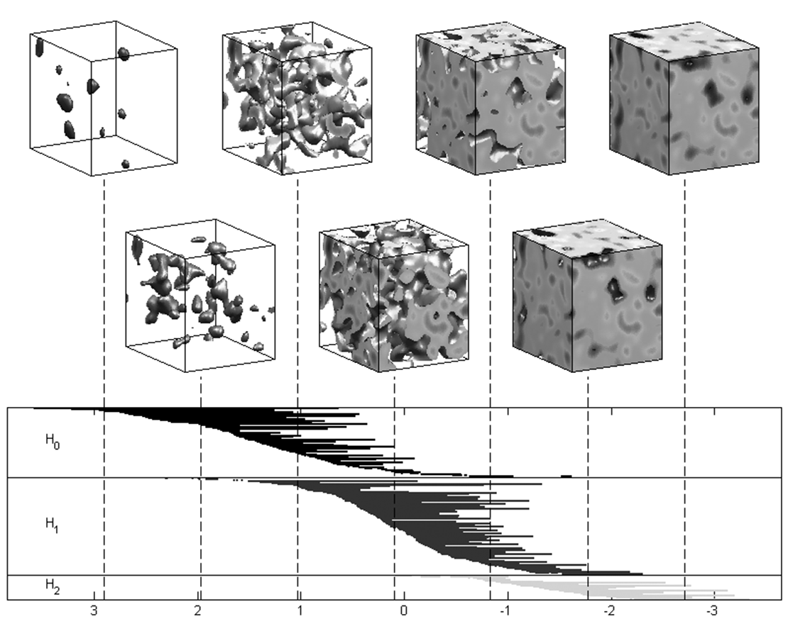
You may recall this figure from Robert’s last column, in which he described the barcodes at the bottom as highly effective Exploratory/Topological Data Analysis descriptors of the three-dimensional structures at the top.
These sets tell you a lot about the function. For example, it is definitely multi-modal, since each of the little regions in the leftmost cubes corresponds to an excursion that must have at least one local maximum somewhere in the middle of it.
Lowering the threshold and moving to the right, the structure of the excursion sets becomes more complicated, and, instead of their being composed of a number of isolated regions, there are fewer regions joined in complicated fashions. In fact, ‘holes’ start to form, of the kind you could poke your finger through if this were a real three-dimensional object rather than a flat representation of one. Moving to the extreme right, almost everything is in the excursion set, and so it now looks like the cube itself, although we can be reasonably certain that there are some small, internal ‘voids’ that must look much like the regions in the left-most cube.
You may not have realized it, but we have just been doing some rather fancy algebraic topology. By talking about isolated regions, holes and voids, we have been talking about the three building blocks that make up all (nice) three-dimensional objects, and we have been following how these change under a filtration. The problem is that, when we move to k-dimensional objects, there are k such building blocks, and nobody really knows what they look like. (In fact, since we can only see in three dimensions, ‘look like’ is probably not even a well-defined term here.)
To get around this, topologists replace these building blocks with algebraic objects, typically groups, and start using terms like kth homology and homotopy to replace holes and voids. It seems almost unbelievable to the novice—including me, even after working with topologists for over half of the last decade—that studying groups and relationships between them could ever be a useful tool for understanding shape. However, not only does this work quite well, but it is the only real tool that Mathematics has for this study, even after more than a century of concentrated effort!
A column like this is hardly the place to define and explain homology theory, but, somewhat amazingly, it is easy to explain something that is intrinsically more complicated, and that is persistent homology. Look again at the cubes in the diagram on the previous page, recall the description above about how things change as we go from left to right, and how regions, holes and voids appear and disappear. Think of this as the ‘birth’ and ‘death’ of the different phenomena, where we morbidly refer to the merger of two as the death of one of them.
The diagram below the cubes encapsulates what I have just written. Each line in the top collection (moving from left to right) illustrates the birth, life, and death of a region, via its starting point, interior, and end point, respectively. The next set of lines do this for the holes, and the lowest set does the same for voids. These lines are typically called bars, and the entire collection a barcode.
Think now of doing this not in our current three-dimensional situation, but in a 1,000-dimensional one. Neither you nor I know what the fourth or 999th topological building blocks look like, but even without this there are numerical algorithms that would allow us to repeat what we just did in three dimensions, and follow the life and death of each one of these structures in a barcode which would now have 1,000, rather than three, regions. In the language of topology, we would be following the persistence of the generators (one per bar) of 1,000 homology groups. You don’t have to understand homology to realize that there is useful information on shape in barcodes.
Life gets even better. Those of you who deal with 1,000 dimensional data know that, typically, the data live on a submanifolds of much lower, and usually single-digit, dimension. That is what techniques of dimension reduction and manifold learning rely on. An interesting, but not surprising, result in algebraic topology is that even if an object has nominal dimension 1,000, if it is really only, for example, three-dimensional, then all the homologies of degree greater than 3 will be empty. In terms of barcodes, there will only be three sets of bars, and the remaining 997 regions will be empty.
So now you can see why applied topologists do it with persistence! Persistent homology, visualized, for example, via barcodes, tells you a lot not only about the dimension of the object you are looking at, but also about its inner structure.
Why don’t theoretical (I refuse to use the honorific ‘pure’ here) topologists do it with persistence? Because, at the turn of the millennium, persistence was invented by applied topologists with a view to applying what they knew to solve real world problems, and … and I will leave you to finish this sentence.
The above example, of analyzing the structure of functions over high dimensional sets has many applications. For example, if the function happened to be a density estimator, then identifying excursion sets would be a way to go about cluster analysis. As opposed to non-topological methods of cluster analysis, this method would tell you not only the number of clusters, but also something about how they sit in relation to one another. Many other applications, including manifold learning, can be found in the references in my previous column. (On persistence itself, especially its computational aspects, see the books by Edelsbrunner and Harer, 2010, or Afra Zomorodian, 2009.)
This month, however, I did not want to concentrate on applications. Rather, I wanted to induct my fellow statisticians and probabilists into the exclusive club of people who use words like ‘homology’ as freely as we say t-test and Chebychev. Now, the next time a topologist throws strange-sounding words at you, you can respond with a sneer and say something deprecating like “Simple homology is so passé. Personally, I do it with persistence”.
Coming up
In the next two columns I want to concentrate on what is missing from the above: randomness. For example, if the function used above for my example is random (e.g. a random field if you are a probabilist, an empirically based density estimator if you are a statistician) then the resulting barcode is also a random object. How a statistician should cope with this in order to draw inferences, or to estimate structures, and how a probabilist might want to generate and analyze random barcodes, are difficult problems, and at the forefront of a lot of current research activity.
Comments on “TOPOS: Applied topologists do it with persistence”